Vocal separation
This notebook demonstrates a simple technique for separating vocals (and other sporadic foreground signals) from accompanying instrumentation.
This is based on the “REPET-SIM” method of Rafii and Pardo, 2012, but includes a couple of modifications and extensions:
- FFT windows overlap by 1/4, instead of 1/2
- Non-local filtering is converted into a soft mask by Wiener filtering. This is similar in spirit to the soft-masking method used by Fitzgerald, 2012, but is a bit more numerically stable in practice.
# Code source: Brian McFee
# License: ISC

##################
# Standard imports
from __future__ import print_function
import numpy as np
import matplotlib.pyplot as plt
import librosa

import librosa.display
Load an example with vocals.
y, sr = librosa.load('audio/Cheese_N_Pot-C_-_16_-_The_Raps_Well_Clean_Album_Version.mp3', duration=120)


# And compute the spectrogram magnitude and phase
S_full, phase = librosa.magphase(librosa.stft(y))
Plot a 5-second slice of the spectrum
idx = slice(*librosa.time_to_frames([30, 35], sr=sr))
plt.figure(figsize=(12, 4))
librosa.display.specshow(librosa.amplitude_to_db(S_full[:, idx], ref=np.max),
                         y_axis='log', x_axis='time', sr=sr)
plt.colorbar()
plt.tight_layout()
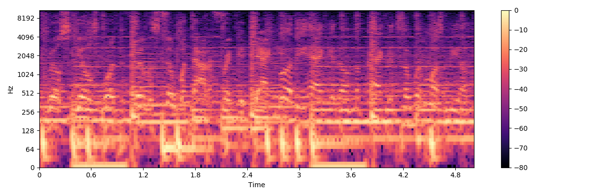
The wiggly lines above are due to the vocal component. Our goal is to separate them from the accompanying instrumentation.
# We'll compare frames using cosine similarity, and aggregate similar frames
# by taking their (per-frequency) median value.
#
# To avoid being biased by local continuity, we constrain similar frames to be
# separated by at least 2 seconds.
#
# This suppresses sparse/non-repetetitive deviations from the average spectrum,
# and works well to discard vocal elements.

S_filter = librosa.decompose.nn_filter(S_full,
                                       aggregate=np.median,
                                       metric='cosine',
                                       width=int(librosa.time_to_frames(2, sr=sr)))

# The output of the filter shouldn't be greater than the input
# if we assume signals are additive.  Taking the pointwise minimium
# with the input spectrum forces this.
S_filter = np.minimum(S_full, S_filter)
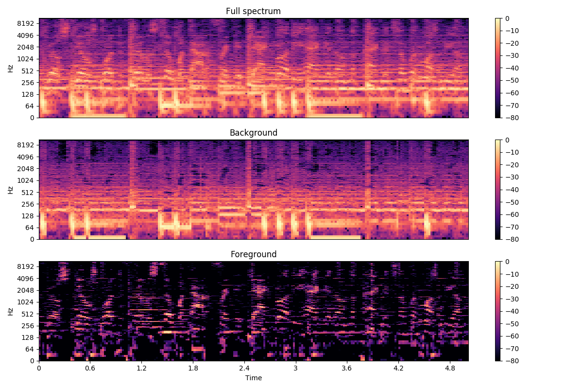
The raw filter output can be used as a mask, but it sounds better if we use soft-masking.
# We can also use a margin to reduce bleed between the vocals and instrumentation masks.
# Note: the margins need not be equal for foreground and background separation
margin_i, margin_v = 2, 10
power = 2

mask_i = librosa.util.softmask(S_filter,
                               margin_i * (S_full - S_filter),
                               power=power)

mask_v = librosa.util.softmask(S_full - S_filter,
                               margin_v * S_filter,
                               power=power)

# Once we have the masks, simply multiply them with the input spectrum
# to separate the components

S_foreground = mask_v * S_full
S_background = mask_i * S_full
Plot the same slice, but separated into its foreground and background
# sphinx_gallery_thumbnail_number = 2

plt.figure(figsize=(12, 8))
plt.subplot(3, 1, 1)
librosa.display.specshow(librosa.amplitude_to_db(S_full[:, idx], ref=np.max),
                         y_axis='log', sr=sr)
plt.title('Full spectrum')
plt.colorbar()

plt.subplot(3, 1, 2)
librosa.display.specshow(librosa.amplitude_to_db(S_background[:, idx], ref=np.max),
                         y_axis='log', sr=sr)
plt.title('Background')
plt.colorbar()
plt.subplot(3, 1, 3)
librosa.display.specshow(librosa.amplitude_to_db(S_foreground[:, idx], ref=np.max),
                         y_axis='log', x_axis='time', sr=sr)
plt.title('Foreground')
plt.colorbar()
plt.tight_layout()
plt.show()
Total running time of the script: ( 2 minutes 53.341 seconds)